Originally published in the Brandywine Asset Management Monthly Report.

Throughout the summer our monthly reports focused on the “perfect” drawdown Brandywine incurred from April through July. We called it perfect because, as we described in those reports, it was right in line with what we expected based on our research and past trading. It was our confidence in our research methodology and the statistical validity of our past performance that led us to write in early July that “now may be an excellent time to invest with Brandywine.”

Another factor that prompted us to recommend new or additional investments was the increase in Brandywine’s market exposure at the end of July. Brandywine employs dozens of fundamentally-based trading strategies, each based on a unique return driver, to trade across more than 150 global financial and commodity markets. When market opportunities arise, an increasing number of those return drivers signal trading opportunities. As a result, our overall portfolio exposure across all strategies and markets is often highest during or immediately prior to our best-performing periods. This is exactly what occurred with Brandywine at the end of July.

During the drawdown (-7.55% over four months), Brandywine’s market exposure, as measured by our margin-to-equity ratio, averaged a below-average 7.81%. We pointed this out in our July report and then wrapped up the discussion by stating that on the last day of July our market exposure (measured by our margin-to-equity ratio) “increased to its highest level in more than four months” and that “this indicates that Brandywine’s Symphony Program is confident about near-term profit opportunities.” July 31 marked the low point in Brandywine’s performance for the year. Since then Brandywine’s Symphony Program has gained +7.10% and our aggressively-traded Brandywine Symphony Preferred Fund gained +30.45%. This rally was accompanied by an average margin-to-equity ratio of 9.59%.

Not every performance drawdown behaves as well as the one we experienced this past summer. And while the odds favored a performance rally at the end of July, there was of course still the possibility that the drawdown could have extended for a longer duration and greater magnitude. All we (Brandywine and our clients) can do is play the percentages, which indicated an approaching end to the drawdown.

Perhaps the best question to ask is, “Why was Brandywine so confident in the percentages?” The answer is due to our use of “Predictive Diversification.”

Predictive Diversification

Predictive Diversification was developed by Brandywine more than twenty years ago. We were systematizing our return driver based trading strategies and sought a process for allocating to each of them in our portfolio. At that time, and remaining to a large extent today, the conventional approach employed by portfolio managers to allocate across the constituents of their portfolios was to use some variation of “mean-variance” modeling such as modern portfolio theory. In this approach, which contributed to Harry Markowitz receiving the Nobel Prize in Economics in 1990, an “efficient frontier” is identified where various allocations result in the best returns for any given level of risk. Unfortunately, this model, although being academically elegant and quite precise, produces results that are simply wrong. Virtually everyone who uses this approach modifies either its inputs or its outputs (such as by using constraints) in order to avoid unrealistic results. They realize that the optimal results derived from the model are unlikely to persist in the future.

Brandywine addressed this issue in the same way we approach all research problems. By starting over. If the output of any of our research projects produces knowingly incorrect results, there is no adequate tweak that can fix it. The project must be redesigned from the start.

In applying this approach to the portfolio diversification problem, we came to realize that modern portfolio theory was the right answer to the wrong question. The question should not have been “How do I solve for the best risk-adjusted return of a portfolio?” The question should have been (and still is!), “How should I allocate within my portfolio in order to achieve the most predictable returns?” (After all, if future performance is knowingly unlikely to match the past, nothing else matters.) It was that question that led to the development of Brandywine’s Predictive Diversification portfolio allocation model. The use of Predictive Diversification, in combination with Brandywine’s return driver based trading strategies, results in portfolio allocations that are significantly different than those produced using conventional portfolio diversification models. But most importantly, Brandywine’s model results in a portfolio that gives us more confidence (than if we had employed conventional portfolio allocation methods) that past performance will carry into the future. After all, that is what we solved for.

If you’re interested in learning more about the unique research philosophy and methodologies that have contributed to Brandywine’s differentiating performance, please contact Rob Proctor or Mike Dever to set up a presentation.

Share this post:

• 
• 
• 

• 
• 
• 
• 
• 
• 
• 
• 
• 
• 
• 
• 
• 
• 
• 

Originally published in the Brandywine Asset Management Monthly Report.

When we began trading Brandywine’s Symphony program in July 2011, we were often asked how we compared to the ‘big names’ in the managed futures industry. While we were friendly and familiar with many of those managers – in fact, Brandywine was either the first or a very early investor in some of today’s largest managers – we didn’t necessarily know the exact nature of how their trading evolved, so we weren’t able to talk specifically about how our approach compared to theirs. But we did have some general knowledge of their trading approaches and so could make some general statements.

The most significant comment we made was that we were confident that our performance would exceed theirs over the next five or ten years. Not out of hubris, but based on some straightforward observations and experience. We didn’t make this statement in any way to malign the other managers, which we respected and continue to respect today. We just felt that we had some distinct advantages that would enable us to outperform. These include:

Size

When Brandywine re-entered the business of trading outside investor money in July 2011, we did so after receiving $10 million in funding from an initial institutional investor. While we have grown since that time, our asset level remains well below that of the largest firms in the business. This provides Brandywine with a size advantage that will persist for a number of years. The two primary benefits of our size are that 1) we are able to easily employ shorter-term trading strategies and 2) we can optimally allocate to less liquid markets that are essentially unavailable to the largest managers. For example, many of our sentiment-based strategies, which have been quite profitable over the past two years, are short-term in nature and difficult to execute by the largest managers. In addition, Brandywine has profited from moves in less-liquid markets, such as the livestock markets, to which the largest managers are unable to optimally allocate.

History

Brandywine’s founder began trading in 1979, and Brandywine was formed in 1982. We managed money for some of the largest managers and, as mentioned in the opening paragraph, were early investors in other leading CTAs. Those early experiences allowed us to explore, observe and execute a tremendous variety of trading approaches. This experience throughout the 1980s served as the basis for the research methodology and investment philosophy that led to the 100% systematic Brandywine Benchmark Program that we traded successfully throughout the 1990s. The consistent performance of the Brandywine Benchmark Program and the resultant increase in our assets under management into the hundreds of millions of dollars were what first led to our recognition as being one of the industry’s leading CTAs.

Research Base

Longevity by itself is not an edge. But during Brandywine’s 30+ years we have innovated and traded numerous unique trading strategies based on sound, logical return drivers. In fact, we pioneered the use of return drivers as being a required basis for a valid trading strategy. Equally important, Brandywine also innovated new portfolio allocation models, such as the “Predictive Diversification” model used by Brandywine over the past two decades. It is these innovations, proven over time with real money at risk, that have contributed to Brandywine’s differentiating performance since the launch of Brandywine’s Symphony Program in July 2011.

The Result

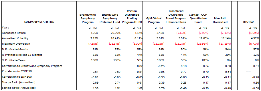
As a result of the investment flexibility provided by Brandywine’s size, our 30+ years of professional experience, and our innovative research, we have been able to fulfill our expectation that we would provide our investors with industry outperformance. This is evidenced in the following chart, which compares Brandywine’s performance to that of the CTAs with which we were most frequently compared when we launched Brandywine’s Symphony Program in July 2011.

Share this post:

• 
• 
• 

• 
• 
• 
• 
• 
• 
• 
• 
• 
• 
• 
• 
• 
• 
• 

Originally published in the Brandywine Asset Management Monthly Report.

Since Brandywine’s Symphony Program began trading in July 2011, it has produced a total gain of +8.79%, while all major CTA indexes have recorded losses (for example, the BTOP 50 lost –4.67% during the period). This past month provides another great demonstration of how Brandywine can profit while other CTAs suffer losses.

The performance difference lies in Brandywine’s Return Driver based investment philosophy and our belief that the most consistent and predictable returns are earned by systematically employing broad strategy and market diversification across a balanced portfolio of fundamentally-based trading strategies. In support of this philosophy, Brandywine employs dozens of independent trading strategies, many of which were first employed by Brandywine more than two decades ago and which continue to be valid today.

A look at some of Brandywine’s trades over the past month provides a great illustration of how these time-tested trading strategies provide Brandywine with differentiating results.

Trade Example #1: Fundamentally-based trade in deferred lean hog market

This trading strategy is highly selective, trading no more than once each year, with more than 70% profitable trades. The original research in support of this strategy was developed in 1991 and the strategy remains valid today.

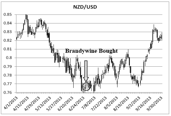
Trade Example #2: Interest rate directional arbitrage in New Zealand Dollar

This trading strategy utilizes interest rate differentials among currencies and within each currency’s yield curve to enter into longer-term positions. The Return Drivers underpinning this strategy are completely independent of trend following, and as you can see on the chart, this presents the opportunity for trades to be entered counter to prevailing trends. The current position was entered on June 27th and has contributed more than 30 basis points of profits to Brandywine’s performance.

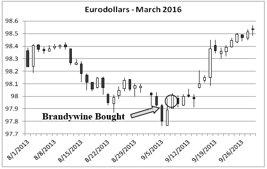
Trade Example #3: Event-driven strategy signal in deferred Eurodollar market

Brandywine’s Event-driven trading strategies trace their roots back to the discretionary trading conducted by Brandywine’s founder in the 1980s. These strategies often take counter-trend positions following the release of government reports or other events. The strategy is selective, entering into approximately one trade per year per relevant market. When the current trade was entered in early September, the Eurodollar market was in a prolonged downtrend. Brandywine’s new long position was counter to that held by trend followers and while already profitable, further benefitted from a strong rally on September 18th following the decision of the U.S. Federal Reserve to delay the start of “tapering.”

With dozens of independent trading strategies trading across well over 100 markets, Brandywine employs more than 1,000 strategy-market combinations similar to those illustrated above. Each of those strategy-market combinations is based on a sound, logical Return Driver with a positive performance expectation that has withstood the test of time. The result is a fundamentally-based investment approach that is balanced across numerous positions and Return Drivers and that is not dependent on any single style of trading or market condition to achieve profits. This is in keeping with Brandywine’s belief that the most consistent and predictable returns are earned by systematically employing broad strategy and market diversification across a balanced portfolio of fundamentally-based trading strategies.

Share this post:

• 
• 
• 

• 
• 
• 
• 
• 
• 
• 
• 
• 
• 
• 
• 
• 
• 
• 

Originally published in the Brandywine Asset Management Monthly Report.

With the U.S. stock market racing to new highs and up almost 150% since the financial crisis low in 2009, we thought it might be a good time to talk about the perception vs. reality in the financial world of the differences between investing and trading. A more complete description of this topic can be found in chapter eight of Mr. Dever’s book, which you can read by following this complimentary link: http://bit.ly/utWsNy.

Investing is often thought of as an act of entering into a position and leaving it on for an extended time. It’s been touted as being the virtuous approach. Trading is the description used to explain the act of changing those positions more frequently. It is considered “speculative’ and often referred to as gambling. The fact is that investing and trading are neither. Investing is the process of identifying the best, most rational opportunities for profiting within your means, and then unemotionally following a process that combines those opportunities into a portfolio that has a high probability of achieving the greatest returns possible while limiting risk over a specific time period. Trading (which involves the development of trading strategies based on disparate “return drivers”) is the method used to achieve that return and thus is a component of investing. In contrast, gambling is entering into or maintaining trades with a negative expected outcome or taking unnecessary risks.

Unfortunately, the process that most people have been taught to follow to earn a return on their money is not investing. It’s gambling. A person who is 60% long stocks and 40% long bonds is taking unnecessary risk. It’s not that there is a problem with being long stocks. It’s that exposing 60% of a portfolio to anything is gambling. That includes government bonds, treasury bills, and other “riskless” investments. The fact is that “angry environments” exist. These are the periods when market conditions are least suitable to any given position. To be in such an environment and not adapt is not smart. In contrast, what people refer to as gambling is often much more akin to trading. For example, a skilled poker player varies her poker play based on the hand she is dealt and the expected behavior of her opponents. She adapts. She’s not a “gambler.” That’s one of the reasons she wins at poker. The same behavior applies to investing. If you put a process in place to ensure that when you’re dealt a “bad hand”, you adapt, you are trading. If you don’t, you’re gambling. Buying and holding stocks through an angry environment is gambling.

Another way to determine if you are gambling, and not investing, is to objectively evaluate your psyche. If you are acutely aware of every fluctuation in the U.S. stock market then you certainly have too much riding on the outcome. You are gambling. If it keeps you up at night then it is a certainty you have too much exposure. If you weren’t gambling on the U.S. stock market you wouldn’t care any more about the movement in U.S. stocks than you would about the movement of orange juice, wheat, oil, or Australian dollars, which are equally tradable for individual investors.

After years of powerful stock market gains, many people, afraid of missing out on further gains such as those that have already been registered, are once again shifting towards gambling behavior by increasing their equity exposure. The memory of the pain inflicted on their portfolios during the dot-com meltdown and the financial crisis has begun to fade. But there are alternatives to long equity exposure that have the potential to produce greater returns – and with less risk – than gambling on a sizable equity position. The fact is that there are a myriad of trading strategies and markets that can be incorporated into an investment portfolio. Picking just a couple, such as being long U.S. equities or long fixed income securities is intentionally limiting and exposes the “poor-folio” to unnecessary and avoidable risks.

Brandywine has spent decades developing a wide range of trading strategies that enable us to diversify our clients’ portfolios across more than 100 global financial and commodity markets. The result is that difficult periods for Brandywine (such as the one we encountered over the past five months) produce relatively constrained losses – certainly relative to the extended and substantial losses experienced by portfolios dominated by long equity exposure. That is because our portfolio is balanced across dozens of return drivers and more than 100 global markets. If you’re interested in learning how you can invest in a truly diversified portfolio, rather than gamble on a poorly-diversified “poor-folio,” give us a call. We look forward to showing you the myriad of ways Brandywine creates a truly globally-diversified portfolio.

Share this post:

• 
• 
• 

• 
• 
• 
• 
• 
• 
• 
• 
• 
• 
• 
• 
• 
• 
• 

Originally published in the Brandywine Asset Management Monthly Report.

Since the end of the first quarter, Brandywine’s Symphony Program has suffered its worst peak-to-trough decline since the start of trading in July 2011. On a daily basis (as opposed to the month-end data usually reported), performance peaked on March 15, 2013 and troughed on July 31, 2013. During that 98 (trading) day period, the program dropped a total of -8.67%. Let’s look at how this compares to expectations based on our tested historical performance.

In the historical simulations for Brandywine’s Symphony Program covering the period January 1999 through June 2011 (immediately prior to the start of actual trading in the program), there were 11 peak-to-trough drawdowns (looking at daily data, not just month-end) that exceeded 8%. This amounts to one such occurrence roughly every 14 months. Based on this data, our current drawdown was a bit overdue, having arrived in our 25th month of actual trading. But what this points out is that, although every drawdown is unwelcome, they will occur, and this current drawdown is right in line with historical expectations.

The key is in controlling drawdowns; limiting their impact so when the turnaround occurs, new performance highs can be quickly achieved. (As Mr. Dever states in the final chapter of his best-selling book, “Drawdowns are the greatest impediment to high returns and are the true measure of risk”). In that regard Brandywine stacks up quite well against the most popular position in most people’s portfolios, the S&P 500. For example, despite being the largest we have incurred, the current drawdown is less than 1/6 that of the S&P 500 decline in 2007 – 2009 and less than 1/5 that of the S&P 500 decline in 2000 – 2002. Brandywine’s Symphony Program controls risk in the following ways:

• Unlike the S&P 500, which in the short-term is dominated by one primary return driver – investor sentiment – Brandywine’s Symphony Program incorporates dozens of trading strategies, based on numerous unrelated return drivers, to trade across more than 100 global financial and commodity markets. This spreads the risk, greatly reducing the impact any single ‘event’ or change in investor sentiment will have on Brandywine’s portfolio. (You can see the primary return drivers powering stock market prices by following this complimentary link to the first chapter of Mr. Dever’s book: http://bit.ly/xrz2Ur).

• Brandywine’s Symphony Program is designed to naturally decrease exposure when there are fewer profit-making opportunities and increase exposure when there are more opportunities. This occurs because Brandywine’s multiple trading strategies operate independently of each other. When there are fewer opportunities, fewer trading strategies signal positions.         
  Evidence of this risk reduction during negative periods is provided by Brandywine’s margin-to-equity ratio, which is a rough measure of market exposure. During down months Brandywine has averaged a M-E ratio of 7.77%, which is more than 15% lower than the ratio during Brandywine’s strongest performing months. Interestingly, (although past performance is not indicative of future performance), Brandywine’s M-E ratio increased to its highest level in more than four months on the last day of July. This indicates that Brandywine’s Symphony Program is confident about near-term profit opportunities.

This confidence reinforces the statement we made last month that “now may be an excellent time to invest with Brandywine.” We believe it is especially opportune for those who have significant investments in the U.S. stock market. Year-to-date, the S&P 500 total return index is up +19.62%. This is significantly above its long-term average (since 1970) of 10.36%. In contrast, Brandywine’s Symphony Program is down 3.00% on the year, while its expected annualized return based on past trading and research is approximately 12%. The divergence is striking and presents a great opportunity for you to diversify your portfolio.

We realize history is not a perfect guide, and past performance is not indicative of future performance, but  – to repeat what we stated last month – if you are prepared to take an analytical—rather than emotional—approach to investing, please call us to discuss how an investment with Brandywine can improve your portfolio’s overall returns and reduce your risk. The time to diversify is now, not after stocks suffer a decline.

Because we reference historical tested performance in this report, the following disclaimer is required:

HYPOTHETICAL PERFORMANCE RESULTS HAVE MANY INHERENT LIMITATIONS, SOME OF WHICH ARE DESCRIBED BELOW. NO REPRESENTATION IS BEING MADE THAT ANY ACCOUNT WILL OR IS LIKELY TO ACHIEVE PROFITS OR LOSSES SIMILAR TO THOSE SHOWN. IN FACT, THERE ARE FREQUENTLY SHARP DIFFERENCES BETWEEN HYPOTHETICAL PERFORMANCE RESULTS AND THE ACTUAL RESULTS ACHIEVED BY ANY PARTICULAR TRADING PROGRAM.

ONE OF THE LIMITATIONS OF HYPOTHETICAL PERFORMANCE RESULTS IS THAT THEY ARE GENERALLY PREPARED WITH THE BENEFIT OF HINDSIGHT. IN ADDITION, HYPOTHETICAL TRADING DOES NOT INVOLVE FINANCIAL RISK, AND NO HYPOTHETICAL TRADING RECORD CAN COMPLETELY ACCOUNT FOR THE IMPACT OF FINANCIAL RISK IN ACTUAL TRADING. FOR EXAMPLE, THE ABILITY TO WITHSTAND LOSSES OR TO ADHERE TO A PARTICULAR TRADING PROGRAM IN SPITE OF TRADING LOSSES ARE MATERIAL POINTS WHICH CAN ALSO ADVERSELY AFFECT ACTUAL TRADING RESULTS. THERE ARE NUMEROUS OTHER FACTORS RELATED TO THE MARKETS IN GENERAL OR TO THE IMPLEMENTATION OF ANY SPECIFIC TRADING PROGRAM WHICH CANNOT BE FULLY ACCOUNTED FOR IN THE PREPARATION OF HYPOTHETICAL PERFORMANCE RESULTS AND ALL OF WHICH CAN ADVERSELY AFFECT ACTUAL TRADING RESULTS.

Share this post:

• 
• 
• 

• 
• 
• 
• 
• 
• 
• 
• 
• 
• 
• 
• 
• 
• 
• 

Originally published in the Brandywine Asset Management Monthly Report.

In Jackass Investing, Mike Dever recounts the story of the siege of Paris in 1871 and the quote made famous at that time when Baron Rothschild told a new investor to “buy securities when there was blood in the streets.” We’ve seen great investors do this time after time. They take advantage of investment opportunities that others are afraid to exploit. But the average person does just the opposite. We know this with certainty (the data is presented in Mr. Dever’s book) and have based a number of Brandywine’s sentiment trading strategies on this return driver. In those strategies Brandywine looks for extremes in market sentiment to take short-term trades opposite the crowd. We apply this approach to both financial (stock indexes, interest rates) and commodity markets. If you’d like to read the chapter where Mr. Dever discusses this (along with an actual trading strategy for trading stock indexes that is revealed in the book’s Action Section), just follow this complimentary link: http://bit.ly/oDQYX8.

The same opportunity can also present itself when evaluating a manager with which to invest. Every investment manager has periods where they outperform and underperform their expected returns. Those managers with less-diversified portfolios tend to have more extreme performances, while those trading more diversified portfolios may have less extreme variations in performance. In the case of Brandywine’s Symphony program, our broad strategy and market diversification has resulted in performance volatility of less than half that of the S&P 500. At the same time we are targeting returns of 12% annually, which is in excess of those to be expected by buying and holding stocks (of course we must remind you that past performance is not indicative of future performance).

But even with a low volatility of returns, Brandywine will regularly incur losing periods. The past three months have been one such period. After reaching new performance highs at the end of March, Brandywine’s Symphony program dropped -4.63% in the 2nd quarter. A drawdown of this moderate size is expected to occur at least once each year. So the question is what to expect going forward. Using history as our guide, we see that similar losing periods are followed, on average, by a positive return of more than 18% (net to our investors) over the subsequent 12 months.

What this points out is that now may be an excellent time to invest with Brandywine. If you follow the approach used by most successful investors, although there is not “blood in the streets” (Brandywine’s diversified approach is intended to avoid such dramatic losing spells), our current drawdown may be a great opportunity to start your investment with Brandywine. In addition to performance, if you have an equity-dependent portfolio, an investment with Brandywine provides tremendous portfolio diversification. The correlation between Brandywine’s Symphony program and the S&P 500 is a (negative) -0.02.

Also, despite the strong rally in stocks and the recent decline by Brandywine, over the past two years the aggressively-traded Brandywine Symphony Preferred Fund has outperformed the S&P 500 (a +17.25% annualized return for Brandywine vs. a +12.77% return for the S&P 500 total return index.

If you are prepared to take an analytical—rather than emotional—approach to investing, please call us to discuss how an investment with Brandywine can improve your portfolio’s overall returns and reduce your risk. The time to diversify is now, not after stocks suffer a decline.

Because we reference historical tested performance in this report, the following disclaimer is required:

HYPOTHETICAL PERFORMANCE RESULTS HAVE MANY INHERENT LIMITATIONS, SOME OF WHICH ARE DESCRIBED BELOW. NO REPRESENTATION IS BEING MADE THAT ANY ACCOUNT WILL OR IS LIKELY TO ACHIEVE PROFITS OR LOSSES SIMILAR TO THOSE SHOWN. IN FACT, THERE ARE FREQUENTLY SHARP DIFFERENCES BETWEEN HYPOTHETICAL PERFORMANCE RESULTS AND THE ACTUAL RESULTS ACHIEVED BY ANY PARTICULAR TRADING PROGRAM.

ONE OF THE LIMITATIONS OF HYPOTHETICAL PERFORMANCE RESULTS IS THAT THEY ARE GENERALLY PREPARED WITH THE BENEFIT OF HINDSIGHT. IN ADDITION, HYPOTHETICAL TRADING DOES NOT INVOLVE FINANCIAL RISK, AND NO HYPOTHETICAL TRADING RECORD CAN COMPLETELY ACCOUNT FOR THE IMPACT OF FINANCIAL RISK IN ACTUAL TRADING. FOR EXAMPLE, THE ABILITY TO WITHSTAND LOSSES OR TO ADHERE TO A PARTICULAR TRADING PROGRAM IN SPITE OF TRADING LOSSES ARE MATERIAL POINTS WHICH CAN ALSO ADVERSELY AFFECT ACTUAL TRADING RESULTS. THERE ARE NUMEROUS OTHER FACTORS RELATED TO THE MARKETS IN GENERAL OR TO THE IMPLEMENTATION OF ANY SPECIFIC TRADING PROGRAM WHICH CANNOT BE FULLY ACCOUNTED FOR IN THE PREPARATION OF HYPOTHETICAL PERFORMANCE RESULTS AND ALL OF WHICH CAN ADVERSELY AFFECT ACTUAL TRADING RESULTS.

Share this post:

• 
• 
• 

• 
• 
• 
• 
• 
• 
• 
• 
• 
• 
• 
• 
• 
• 
• 

For the past 31 years[i], a conventionally-diversified portfolio consisting of 60% stocks and 40% bonds has provided investors with satisfying returns of +10.80% annually. This was the result of both stocks and bonds advancing strongly throughout that period. Better yet, stocks and bonds complimented each other nicely. When stocks returned +19.35% annually from the market low in 1982 to its peak in August 2000, bonds lagged somewhat (although still returning a substantial +10.34% annually). But in the period from the 2000 market peak to the 2009 market low, while stocks declined a sharp -43.51%, bonds balanced that with a strong +61.78% rally. More recently, both stocks and bonds have advanced, with the 60-40 portfolio gaining an annualized +15.36% from the market low in March 2009 to May 31, 2013.

The past 31 years was an unprecedented period for a 60-40 portfolio; one that wasn’t seen prior. In fact, as I wrote in my best-selling book, Jackass Investing: Don’t do it. Profit from it., “all of the real stock market returns over the past 111 years can be attributed to just an 18 year period – the great bull market that began in August 1982 and ended in August 2000. Without those years the real, inflation-adjusted return of stocks, without reinvesting dividends, was negative.”

Unfortunately for investors, the 60-40 results of the past 30 years aren’t likely to repeat in the near future. Here’s why not.

Return drivers for U.S. equities

There’s an ethos among equity investors that stocks provide an intrinsic return. This ethos is rooted in a depth of academic research that identifies an equity “risk premium” as the source of stock market returns. The equity risk premium is the “theory” that equities are destined to produce greater returns than less risky investments such as corporate bonds, simply because they ARE riskier.

In fact, the “research” supporting the equity risk premium is actually not research at all but merely an observation – an observation that over the past couple of centuries stock returns outperformed bonds. Then a postulate, the risk premium, was created to support that observation, which in turn was “proven” by the observed data. As you could likely surmise from the obvious circularity of the postulate and proof, this is wrong. The risk of investing in stocks has nothing at all to do with their returns. As I show in Jackass Investing, stock market returns are driven by three primary “return drivers”.

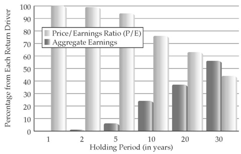
In the book’s first chapter I show how over the long term stock market returns are dominated by corporate earnings growth, and in the short-term (less than 20 years) by the multiplier (the “price/earnings” or “P/E” ratio) people are willing to pay for those earnings. The chart displaying this is reproduced here[ii]:

In the second chapter I display the fact that historically, dividends have provided 48% of the total return from U.S. equity investing over the period 1900 – 2010[iii]. (In most of the studies presented in my book and in this article, I use the S&P 500 total return index which includes dividends. The ETF that generally corresponds to the price and yield performance of the S&P 500 is SPY).

Knowing this, these were the three dominant return drivers that contributed to the stock market’s +11.88% annualized return over the past 31 years:

1. 6.16% of the annual return was driven by the average annual profit growth of 6.16%
2. 3.19% of the annual return was the result of the increase in the P/E ratio from 10 in 1982 to more than 23 at the end of 2012 (using the cyclically-adjusted P/E (“CAPE”) presented by Robert Shiller in his book Irrational Exuberance[iv])
3. 2.53% of the annual return was due to the dividend rate starting the period at an historically high 6.24% in 1982 and averaging 2.53% throughout the period

Going forward, if the P/E ratio reverts to its long-term average of 16.4, corporate profits grow at their historical average of +4.70%, and dividends increase at the same rate as corporate profits (and the dividend payout ratio increases to its long-term average), stocks will appreciate at just 7.05% per year over the next decade. Here’s the arithmetic.

Future returns from U.S. equities

To determine the likely return for the S&P 500 over the remainder of this decade we need three primary inputs:

1. The rate of earnings growth for the companies underlying the index,
2. The most likely P/E ratio people will pay for those earnings at year-end 2020, and
3. The dividend yield for those stocks during the period.

Let’s look at each of these in turn.

Return contribution from earnings growth

Since 1900, the nominal (before inflation) average annual growth rate for companies in the S&P 500 has been 4.7%. Over the same period the average annual inflation rate has been 3.04%. For purposes of our projections I will assume these two variables continue at the same rates into the future. While I understand there are many people who expect a substantial increase in inflation, historically, that has also resulted in an increase in the nominal (before inflation) return for the S&P 500. So if that were to occur, while the nominal return from the S&P 500 would likely increase, the real (after inflation) rate of return would, on average, remain around the historical level of 1.7%. Because of this, I project the annual return contribution from earnings growth, between 2012 and the end of 2020, will be +4.70%.

Return contribution from investor sentiment

There are a variety of methods used to calculate the price/earnings ratio of a stock or stock index. The method I will use in this article is CAPE (“Cyclically Adjusted Price Earnings Ratio”), the ratio popularized by Robert Shiller in his book Irrational Exuberance. CAPE compares the S&P 500’s current price to the 10-year average of earnings. This has the benefit of smoothing earnings volatility to reduce the short-term impact of events such as the 2008 financial crisis. Over the past 113 years, CAPE has ranged from a low of 4.46 (in the depths of the Great Depression) to a high of 48.94 (at the peak of “dot-com” hysteria in 1999). The average CAPE over that period has been 18.63.

As of year-end 2012 CAPE stood at 23.37. Part of the reason the rate was above the long-term average was because the 10-year average earnings value used in the calculation was depressed by the effects of the Great Recession of 2008. In order to make the CAPE value in 2020 appear less elevated (compared to the long-term average) than it appears today due to the Great Recession, I will continue to walk forward the earnings average of the prior 10 years from 2013 through 2020, assuming average earnings growth based on the long-term average of 4.7%. This results in a growth rate of 6.8% for the 10-year earnings average from 2013 through 2020.

As a result of the combination of the increase in the 10-year average of profit growth and CAPE reverting to its long-term average, I project the annual return contribution from investor sentiment, between 2012 and the end of 2020, will be -0.72%.

Return contribution from dividends

The dividend yield on the S&P 500 at year-end 2012 was approximately 2.20%. This represents a dividend payout ratio of 36%. This figure is quite a bit lower than the 113 year average of 59%. If the payout ratio reverts to its long-term average, this will boost the dividend yield over the remainder of this decade. As a result of this, and assuming that dividends grow at the same rate as profits, which is 4.7% per year, I project the annual return contribution from dividends, between 2012 and the end of 2020, will be +3.07%.

Calculating the S&P 500 total return

We’re now left with a simple arithmetic problem to determine the projected average annual return for the S&P total return index, between 2012 and the end of 2020.

This is the sum of the contribution from each of the three return drivers:

Future returns from bonds

For the past 31 years the Barclay Aggregate Bond Index averaged annualized returns of 8.43%. Unfortunately, the two primary return drivers that contributed to that performance are both destined to provide much lower returns in the future. They are:

1. The capital appreciation provided as the high interest rate of 13% that prevailed at the start of the period declined to just over 1% today, and
2. The average yield of 5.74% on the 5-year Treasury note over the period.

With the Barclay Aggregate Bond Index now yielding just over 2%, and the U.S. Treasury 5-year note yielding 1.05%, the likely return from bonds over the remainder of this decade should be similar to the current yield on the Barclay Aggregate Bond Index, which, as represented by the iShares ETF (AGG) is 2.43%.

Calculating the return on the 60-40 portfolio

In summary then, based on the above straightforward analysis, from year-end 2012 through year-end 2020 we can expect the following return from a conventional 60-40 portfolio:

This is less than 1/2 the return earned over the past 31 years and approximately 1/3 the returns produced since the Great Recession low in March 2009. As I pointed out at the beginning of this article, 60-40 has always been a risky proposition; returns are earned in a “lumpy” fashion. Without the tailwinds of low P/E, high dividend yield and high interest rates, in the future those lumpy returns will be earned in relation to a lower trendline of overall performance. Also, while these projections are based on a sound analysis of the return drivers powering the 60-40 portfolio’s performance, they are certainly not absolute. Already, in the first 5 months of the 8-year projection period (January 2013 through December 2020), the 60-40 portfolio has gained more than 5%, twice that expected from these projections.

Portfolio diversification is the one true “free lunch” of investing, where you can achieve both greater returns and less risk. But, as can be seen by its reliance on just four return drivers, the conventional 60-40 portfolio does not provide true portfolio diversification. When those four return drivers underperform, as is indicated by the projections in this article, performance will suffer. True portfolio diversification can only be obtained by increasing diversification across dozens of return drivers. I give examples of a truly diversified portfolio in the final chapter of my book, and am pleased to provide a complimentary link to that chapter here: Myth 20. While some people may prefer to gamble on a less-diversified 60-40 portfolio, as my book shows, in the longer-term, true portfolio diversification can lead to both increased returns and reduced risk.

————————————————–

[i] From the market low at the end of July 1982 through May 31, 2013.

[ii] Michael Dever, Jackass Investing: Don’t do it. Profit from it. (Thornton: Ignite Publications, 2011).

This study uses linear regression analysis to determine the degree to which variance in the S&P 500 Total Return Index over various holding periods (1, 2, 5, 10, 20 and 30 years) was explained by the changes in nominal earnings and changes in P/E. A 10 year average was used to represent both the nominal earnings and the “E” in the P/E in order to reduce the impact of economic cycles. The regression analysis included three separate regression calculations for each holding period. The first regression measured the goodness of fit for changes in average earnings versus S&P total returns. The second regression measured the goodness of fit for changes in the P/E versus S&P total return. The third regression includes the two parameters, average earnings and P/E, versus S&P 500 total returns. Since linear regression assumes orthogonality of the independent variables, that assumption was tested on all of the holding period data. The Percentage change in the nominal earnings versus the P/E ratio had R2 values ranging from 2% to 6% across all holding periods, suggesting the two regression parameters are mostly independent of each other. Furthermore, the two parameter regressions were found to explain greater than 93% of the variance in the S&P 500 total return over each holding period. Since nearly all of the variance in the S&P 500 return is captured by the two parameter regression I normalized the R2 result from each of the single parameter regressions to 100% for use in Figure 3. The use of the single parameter R2 to measure the explanatory power of the S&P 500 total return for the two regression variables is an approximation. The subtle (

[iii] Annualized return of S&P 500 TR index 1900 – 2010: +9.51%. Annualized return of S&P 500 w/o reinvesting dividends: +4.92%. Contribution of dividends = (9.51 – 4.92) / 9.51 = 48%.

[iv] The cyclically-adjusted P/E (“CAPE”) used by Robert Shiller in his book: Robert J. Shiller, Irrational Exuberance (Princeton: Princeton University Press, 2000, 2005, updated). Data used in Shiller book and for S&P 500 Total Return performance available at: http://www.econ.yale.edu/~shiller/data/ie_data.xls. Retrieved February 14, 2011.

[v] This was the rate on the 5 year U.S. government bond. Five years is used as that is the approximate average duration of the Barclay Aggregate Bond Index.

Share this post:

• 
• 
• 

• 
• 
• 
• 
• 
• 
• 
• 
• 
• 
• 
• 
• 
• 
•